


Sesame (Sesamum indicum) is one of the important summer crops in Korea. But annual sesame production gradually reduced up to 12,421 metric tons in 2013 compared to 31, 859 metric tons in 1995. In addition, the self-sufficiency rate of domestic sesame was also sharply decreased up to about 15%. Sesame is originated form Africa savanna area, and meteorological factors such as temperature, rainfall and amount of solar radiation determine yield potential of sesame. Usually, sesame grows from middle of May to early of September in Korea and occasionally, heavy rain and typhoon give damage to the sesame productivity. Therefore, it is very important for sesame breeder to select optimum cultivation region to minimize environmental factors and maximize genotypic effects. Genotype main effect and genotype by environment interaction (GGE) biplot analysis is one of methods to determine sesame yield stability and select suitable variety in different environments. Comparisons of varieties at different environments may results in high genotype by environment (G x E) interaction (Fehr, 1987). AMMI is especially effective tool where the assumption of linearity of the response of genotype to a change in the environment is not fulfilled (Allard et al., 1964; Zobel et al., 1988; Yan and Hunt, 1998) and which usually separates the interaction part of the multiplicative components into the additive main effects by principal component analysis. The GGE biplot analysis has several biplot interpretation methods, in which genotype and test environment evaluation can be visually addressed (Yan and Rajcan, 2002; Yan and Kang, 2003; Yan and Tinker, 2006; Pourdad and Moghaddam, 2013). Therefore, GGE biplots were widely used for plant breeders to analyze mega environment evaluation. AMMI and GGE models help to understand complex genotype by environment (G × E) interactions, and in turn, determine which genotype has been in which environments, and also help when grouping environments with the similar winners into mega environments(Pourdad and Moghaddam, 2013). The objective of the present study was to identify the suitable sesame genotypes with both mean performance and high stability, and to demonstrate the application of the GGE biplot analysis to determine sesame yield stability.
MATERIALS AND METHODS
Plant materials and experimental environments
This experiment was conducted at the eight sites of Miryang, Suwon, Chuncheon, Cheongwon, Yeasan, Iksan, Andong and Naju areas from 2013 to 2014. Total ten sesame varieties, Yangbaek, Ansan, Kopoom, Kanghuk, Miryang47, Miryang48, Miryang49, Miryang50, Kyeongbuk18 and Kyeongbuk19 were used for this experiment. The experimental plot size was about 12m2. A black polyethylene film with 30 x 10 cm hole space was mulched and sown the seed in a mulched film hole. Finally, the young seedlings were thinned to make one plant per hole. Basic fertilizer (N-P2O5-K2O=8-4-9) was applied as the basal condition. Meteorological data of eight different experimental sites were analyzed in two years (Table 1). Year 2014 showed relatively higher temperature and solar radiation amount rather than year 2013. Especially, Southern regions, such as Miryang, Naju recorded hot weather condition(relatively higher temperature and solar radiation) among eight sites and rainfall amount showed widely different depending on the experimental sites.
Table 1.
Meteorological data of eight different experimental sites in 2013~2014.
Combination of average grain yield of two years (2013 and 2014) with eight sites were treated as eight environments (Table 2). Generally, grain yield in a given environment was determined by the effect of genotypes (G), environments (E) and genotype x environment interaction (G x E). Therefore, the yield responses of genotype were different depending on the extend of environments and genotype x environment interaction effects. For more detailed analysis of the interactions, the additive main effect and multiplicative interaction (AMMI) model analysis, or genotype main effect and genotype by environment interaction (GGE) biplot analysis is required.
Table 2.
Average grain yields (kg/10a) of ten sesame genotypes across the eight experimental sites in 2013~2014.
| Genotypes | Environments | ||||||||||
|---|---|---|---|---|---|---|---|---|---|---|---|
| Miryang | Suwon | Chuncheon | Cheongwon | Yeasan | Iksan | Naju | Andong | Mean | S. D.a | C. V.b | |
| Yangbaek | 104 | 107 | 117 | 124 | 127 | 93 | 120 | 102 | 112 | 11.99 | 0.11 |
| Ansan | 84 | 121 | 107 | 105 | 152 | 80 | 115 | 73 | 105 | 25.80 | 0.25 |
| Kopoom | 73 | 112 | 105 | 102 | 149 | 94 | 113 | 61 | 101 | 26.78 | 0.28 |
| Kanghuk | 99 | 86 | 75 | 103 | 117 | 97 | 95 | 91 | 95 | 12.33 | 0.13 |
| Miryang47 | 115 | 102 | 122 | 142 | 95 | 120 | 102 | 115 | 114 | 14.81 | 0.13 |
| Miryang48 | 121 | 99 | 102 | 132 | 159 | 99 | 122 | 105 | 117 | 20.86 | 0.18 |
| Miryang49 | 122 | 99 | 95 | 109 | 86 | 106 | 83 | 102 | 100 | 12.62 | 0.13 |
| Miryang50 | 113 | 126 | 96 | 108 | 140 | 100 | 109 | 75 | 108 | 19.53 | 0.18 |
| Kyeongbuk18 | 104 | 122 | 96 | 124 | 138 | 90 | 131 | 111 | 115 | 17.05 | 0.15 |
| Kyeongbuk19 | 114 | 85 | 74 | 131 | 130 | 92 | 103 | 102 | 104 | 20.41 | 0.20 |
| Mean | 105 | 106 | 99 | 118 | 129 | 97 | 109 | 94 | - | - | - |
| S. D. | 15.96 | 14.42 | 15.62 | 14.31 | 24.00 | 10.60 | 14.07 | 18.08 | - | - | - |
| C. V. | 0.15 | 0.14 | 0.16 | 0.12 | 0.18 | 0.11 | 0.13 | 0.19 | - | - | - |
Methods of statistical analysis and those application
AMMI model is expressed by Yij=μ + gi + ej + Σλkγikδjk+εij, where Yij is the yield of i-th genotype in the j-th environment; μ is the grand mean; gi and ej are the deviations of genotype and environment from the grand mean, respectively. λk is the eigenvalue of the principal component analysis (PCA) for axis k; γik and δjk are the genotype and environment principal components scores for axis k; N is the number of principal components in the AMMI model; εij is the residual term. Genotype and environment PCA scores are expressed as unit vector times the square root of λk (genotype PCA score=λkδik, environment PCA score=λkδik, (Zobel et al., 1988)). To interpret G x E interaction, correlation analysis was conducted between genotypic and environmental scores of the first and second interaction principal component axes (IPCA1 and IPCA2) from the AMMI model. ANOVA (Analysis of Variance) analysis was conducted to determine the effects of genotype x environment interaction. Software (AMMI) model and GGE biplot analysis package was used to analyze the data visually in the windows environment. Angels drown between environment vectors were used to determine correlations (similarities) between environment pairs in the GGE biplot analysis (Yan and Kang, 2003). GGE distance was used to determine correlation with yield stability statistics.
RESULTS AND DISCUSSION
Comparison of agronomic characteristics of sesame genotypes under different environments
Genotype Miryang47 and Kyeongbuk18 showed higher average grain yield among genotypes under different environments (Table 2). Cheongwon and Yeasan were better sites in terms of grain yield comparison. According to the basic statistical analysis, Cheongwon and Iksan showed relatively smaller standard deviation and coefficient variation value probably due to small portion effect of environments (E) and genotype x environment interaction (G x E).
Analysis of variance of genotypes, environments and G x E with AMMI model
Analysis of variance was conducted to determine the effect of genotypes (G), environments (E) and genotype x environment interaction (G x E). The results were shown in Table 3. AMMI analysis of variance indicated that three multiplicative terms were significant (P<0.05). Grain yield of sesame genotypes was significantly affected by environment which explained 61% of the total variation, whereas genotype and genotype x environment interaction were explained 16%, 24% respectively. The AMMI model partitioned G x E interaction effects into successively specific patterns. Partitioning of G x E indicates that AMMI-4 model describes the G x E patterns for yield by the first four interaction principal component analysis (IPCA) scores using Gollb's F-test. Of the total variations, about 24% is due to G x E interaction effects, and 76% is due to the genotype and envi ronmental effects which are explained by additive main effect.
Table 3.
Analysis of variance with interactive model(a) and partitioning interaction with AMMI (b) of average grain yield per ten are of sesame genotypes across eight environments.
(a)| Source of variation | df | Sum of Squares | Efficiency (%) | Mean Squares | F-test |
|---|---|---|---|---|---|
| Total | 79 | 36987.80 | 100.0 | ||
| Genotype | 9 | 5811.64 | 15.7 | 645.74 | ** |
| Environment | 7 | 22380.60 | 60.5 | 3197.22 | ** |
| G x E | 63 | 8795.57 | 23.8 | 139.61 | * |
Graphical statistical methods based on GGE biplot analysis
Environment centered GGE biplot was used to estimate the pattern of environments in Fig. 1. Environment PC1 score showed both negative and positive values indicating different response of yield performance among genotypes across environments due to the effect of G × E interactions. Environment PC2 scores also showed both positive and negative scores. This meant to make some G x E interaction effect, leading to inconsistent genotype yield performance across the eight environments. To compare the relationship between environments, some lines are drawn to connect the test environments to the biplot origin as environment vectors. The angle cosine between two environments is used to the extent of the correlation between them(Kroonenburg, 1995; Yan and Tinker. 2006; Dehghani et al., 2010). For example Andong, Miryang and Chuncheon were positively correlated (an acute angle), Yeasan and Cheongwon were negatively correlated (an obtuse angle) in Fig. 1. The presence of wide obtuse angle (strong negative correlations) among environments is an indication of high cross over GEI (Yan and Tinker, 2006).
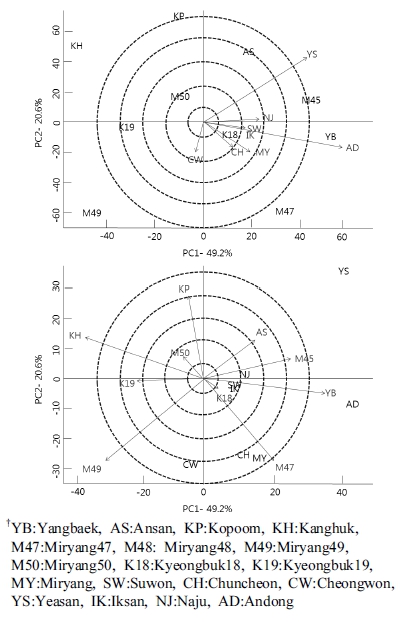
Fig. 1.
Vector view of GGE biplot of environment-focused scaling(left) and genotype-focused scaling(right) of average grain yield per ten are of sesame genotypes across eight environments.The distance between two environments or genotypes measures their dissimilarity in discriminating the genotypes or environments. On the left side of Fig. 1, Miryang, Suwon, Chuncheon and Andong get the position in the first group while Yeasan and Cheongwon separately form their own group. Close associations among some locations indicate that some information about genotypes could be obtained from fewer test locations, and it would reduce test cost (Choukan, 2010). Likewise, Ansan and Miryang45 showed same group position(right side of Fig. 1). Otherwise, Koppoom, Miryang50 and Kanghuck showed different group from previous two genotypes. Vector of GGE biplot in the genotype focused scaling also measures their dissimilarity in discriminating the genotypes among environments, but the accuracy of dissimilarity is not always expected because the biplot didn’t explain 100% of the GGE variation.
Discriminating ability and representativeness of the test environment
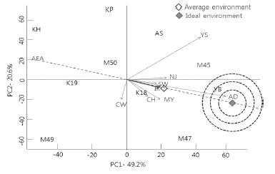
Discriminating ability and representativeness of the testing environments are an important measure in the GGE biplot. The concentric circles as shown in Fig. 2 help to visualize the length of the environment vectors, which are a measure of the discriminating ability of the environments as well as standard deviation within the respective environments. According to the result, Yeasan and Andong were most discriminating (informative). Otherwise, Naju, Iksan and Suwon showed least discriminating. Test environments that are consistently non discriminating provide little information on the genotypes, in which is inappropriate as test environments. The average environment which is drawn as small circle at the end of the arrow in Fig. 2 has the average coordinates of all test environments, and Average Environment Axis (AEA) is the line passing through the average environment and the biplot origin. A test environment showing a smaller angle with the AEA is more representative than other test environments (Yan and Rajcan, 2002). Thus, Suwon, Iksan, Andong and Naju are most representative whereas Yeasan and Cheongwon least representative. Test environments with both discriminating and representative are good test environments for selecting generally adaptable genotypes. Discriminating but non representative test environments like Yesan are useful for selecting specifically adaptable genotypes if the target environments can be divided into mega environments or they are useful for culling unstable genotypes if the target environment is a single mega environment.
Mean performance and stability of genotypes
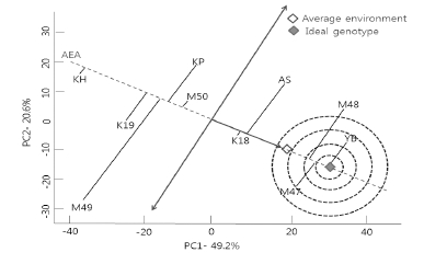
Fig. 3 presents the biplot of stability and mean performance of ten genotypes. The small tetragon indicates average environment defined by the intercept of PC1 and PC2 scores of the environment. According to the Fig. 3, the line that passes through the biplot origin and the average environment with single arrow is the Average Environment Axis (AEA). Projections of genotype markers to the average environment axis show the mean yield of genotypes. Thus, genotypes are ranked along the ordinate. Genotype Yangbaek was highest yielding genotype on average while Kanghuk was lowest yielding genotype. The AEA ordinate is the double arrowed line that passes through the biplot origin and is perpendicular to the AEA abscissa. The AEA ordinate approximates the G x E interaction associated with each genotype and this is a measure of variability or instability of the genotypes. Greater projection onto AEA ordinate, regardless of the direction means greater instability. Therefore, genotypes Miryang49, Koppoom and Ansan are unstable. Whereas, Kyeongbuk18, Miryang50 and Kanghuk which showed shorter projections were relatively stable over the environments. The genotypes that combined good performance with stability include Yangbak because it is closeness to the mean yield and short projection of the genotype marker lines.
Visualization of Which-Won-Where Pattern in Multi-Environments
The which-won-where pattern of multi-environment data is necessary to analyze the possible existence of different environments in a region(Gauch and Zobel, 1997; Yan, 2001). Fig. 4 displays the polygon view of a GGE biplot with which-won-where pattern. The polygon is drawn on genotypes relatively remote from the biplot origin so that all genotypes are contained within the polygon. The lines in Fig. 4 were formed as perpendicular to the sides of the polygon or their extensions. These perpendiculars divide the biplot into several sectors. Line 1 was perpendicular to the side that connects genotypes Ansan and Koppoom; Line 2 was perpendicular to extension of Koppoom and Kanghuk; Line 3 was perpendicular to side Kanghuk and Miryang49; Line 4 was perpendicular to side Miryang49 and Miryang47; Line 5 was perpendicular to side Miryang47 and Yangbaek. There are five sectors and the environments fall into three of them. The environment group within each sector and the genotypes at the polygon’s extremity characterized the mega environment (Yan and Rajcan, 2002). Thus, three mega environments were characterized, one with Yeasan, Naju, Suwon, Iksan and Andong is grouped as one mega environment, while environment Chuncheon and Miryang were grouped as another mega environment. The genotypes located at the sector’s vertex had optimum performance in their respective mega environment. Thus, Ansan, Miryang48 and Yangbaek had better performance in the environment of Naju, Suwon, Iksan and Andong. Similarly, genotype Miyrang47 exhibited better performance in the environments of Chuncheon and Miryang.

CONCLUSION
Miryang, Suwon, Chuncheon and Andong get the similar position in the first group, while Yeasan and Cheongwon separately form another their own group. The AEA ordinate approximates the G x E interaction associated with each genotype and this is a measure of variability or instability of the genotypes (Asnake et al., 2013). Genotype Miryang49, Koppoom and Ansan are unstable. Whereas, Kyeongbuk18, Miryang50 and Kanghuk which showed shorter projections were relatively stable over the environments. From GGE point of view, the eight environments were grouped into five mega environments, Three mega environments were characterized as follows; one with Yeasan, Naju, Suwon, Iksan and Andong is grouped as one mega environment, while environment Chuncheon and Miryang were grouped as another mega environment. According to GGE interpretation, an ideal test environment should be both discriminating and representative. An ideal environment probably does not exist in reality but can be used as a reference point. From our study result, it can be seen that Andong is the closest to the ideal environment, and therefore, is the most desirable of the eight environments. Ansan, Miryang48 and Yangbaek had better performance in the environment of Naju, Suwon, Iksan and Andong. Similarly, genotype Miyrang47 exhibited better performance in the environments of Chuncheon and Miryang. In conclusion, It showed that the GEI biplots were effective enough for visualizing the response patterns of genotypes and environments.